Overview
This dataset include the geochemistry data of 1711 silt samples and 55 variables within each samples. For each sample, the Easting and Northing coordinates under Universal Transverse Mercator system (UMT) were recorded for mapping purpose (not regarded as variables) in the data table. The 55 variables are the metal and non-metal elements content in every single silt sample collected form Mackenzie Mountain. As mentioned in previous web page, the values of each variable are the results of best validity after comparing the raw data from ICP, ICPES, ICPMS, AAS and INAA tests. Table 1 below displayed the header, first 6 variables of each sample and first/last 6 samples of the entire data set.
This dataset include the geochemistry data of 1711 silt samples and 55 variables within each samples. For each sample, the Easting and Northing coordinates under Universal Transverse Mercator system (UMT) were recorded for mapping purpose (not regarded as variables) in the data table. The 55 variables are the metal and non-metal elements content in every single silt sample collected form Mackenzie Mountain. As mentioned in previous web page, the values of each variable are the results of best validity after comparing the raw data from ICP, ICPES, ICPMS, AAS and INAA tests. Table 1 below displayed the header, first 6 variables of each sample and first/last 6 samples of the entire data set.
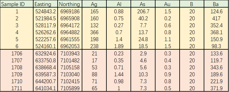
Table. 1 Raw Data Display (after data selection)
Data Cleaning and Transformation
After data selection, data set can still create problems during the multivariate analysis. Meanwhile, “outliers” always pop out when performing ordination tools. Before multivariate analysis, descriptive statistics were performed to help cleaning the potential “problematic” data out and choosing the proper data transformation types.
In this data, variable Ge and Ta results are the same for all samples, so the Ge and Ta data are cleared out. There are also outliers with extremely high or low values in some samples comparing to values in other samples. These values were kept for the first time running of multivariate analysis but may be replaced with the average of rest of data within the sample in later runs.
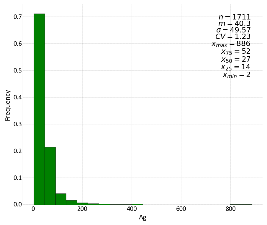
It will be too many figures if histograms of all 53 variables are displayed. In figure 5-1, 5-2, 5-3, histograms of three variables from the data set are displayed to show the distribution of original data. It is obvious that for all the variables we had in the data set are positive skewed with long tails.
In figure 6-1, 6-2, 6-3, histograms of log transformed data of variable Ag, Mn and Pb are displayed, showing better normality.
After data selection, data set can still create problems during the multivariate analysis. Meanwhile, “outliers” always pop out when performing ordination tools. Before multivariate analysis, descriptive statistics were performed to help cleaning the potential “problematic” data out and choosing the proper data transformation types.
In this data, variable Ge and Ta results are the same for all samples, so the Ge and Ta data are cleared out. There are also outliers with extremely high or low values in some samples comparing to values in other samples. These values were kept for the first time running of multivariate analysis but may be replaced with the average of rest of data within the sample in later runs.
It will be too many figures if histograms of all 53 variables are displayed. In figure 5-1, 5-2, 5-3, histograms of three variables from the data set are displayed to show the distribution of original data. It is obvious that for all the variables we had in the data set are positive skewed with long tails.
In figure 6-1, 6-2, 6-3, histograms of log transformed data of variable Ag, Mn and Pb are displayed, showing better normality.